
R code for example in Chapter 8:
Fitting probability models to frequency data
New methods on this page
These are the core commands that produce the new methods described in Chapter 8. The variable names are plucked from the examples further below.
- \(\chi^2\) goodness-of-fit test:
chisq.test(birthDayTable, p = c(52,52,52,52,52,53,52)/365))- Calculate Poisson probabilities:
dpois(0:20, lambda = meanExtinctions)Other new methods:
Divide individuals into groups based on a numeric variable using cut.
Examples
Example 8.1. Birth days of the week
Fit the proportional probability model to frequency data.
Read and inspect the data. Each row represents a single birth, and shows the day of the week of birth.
birthDay <- read.csv("../Data/chapter08/chap08e1DayOfBirth.csv")
head(birthDay)
## day
## 1 Sunday
## 2 Sunday
## 3 Sunday
## 4 Sunday
## 5 Sunday
## 6 SundayPut the days of the week in the correct order for tables and graphs.
birthDay$day <- factor(birthDay$day, levels = c("Sunday", "Monday",
    "Tuesday", "Wednesday","Thursday","Friday","Saturday"))
Frequency table of numbers of births (Table 8.1-1).
birthDayTable <- table(birthDay$day)
data.frame(Frequency = addmargins(birthDayTable))
## Frequency.Var1 Frequency.Freq
## 1 Sunday 33
## 2 Monday 41
## 3 Tuesday 63
## 4 Wednesday 63
## 5 Thursday 47
## 6 Friday 56
## 7 Saturday 47
## 8 Sum 350Bar graph of the birth data. The argument cex.names = 0.8 shrinks the names of the weekdays to 80% of the default size so that they fit in the graphics window – otherwise one or more names may be dropped.
barplot(birthDayTable, cex.names = 0.8)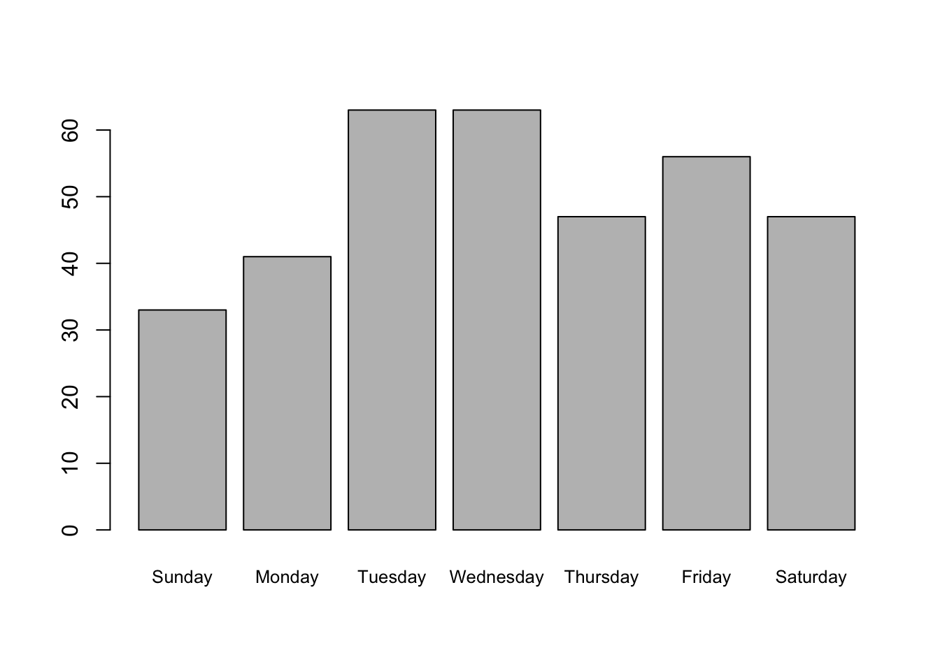
Commands for a bar graph with more options (Figure 8.1-1) are given here.
shortNames = substr(names(birthDayTable), 1, 3)
barplot(table(birthDay$day), names = shortNames,
ylab = "Frequency", las = 1, col = "firebrick")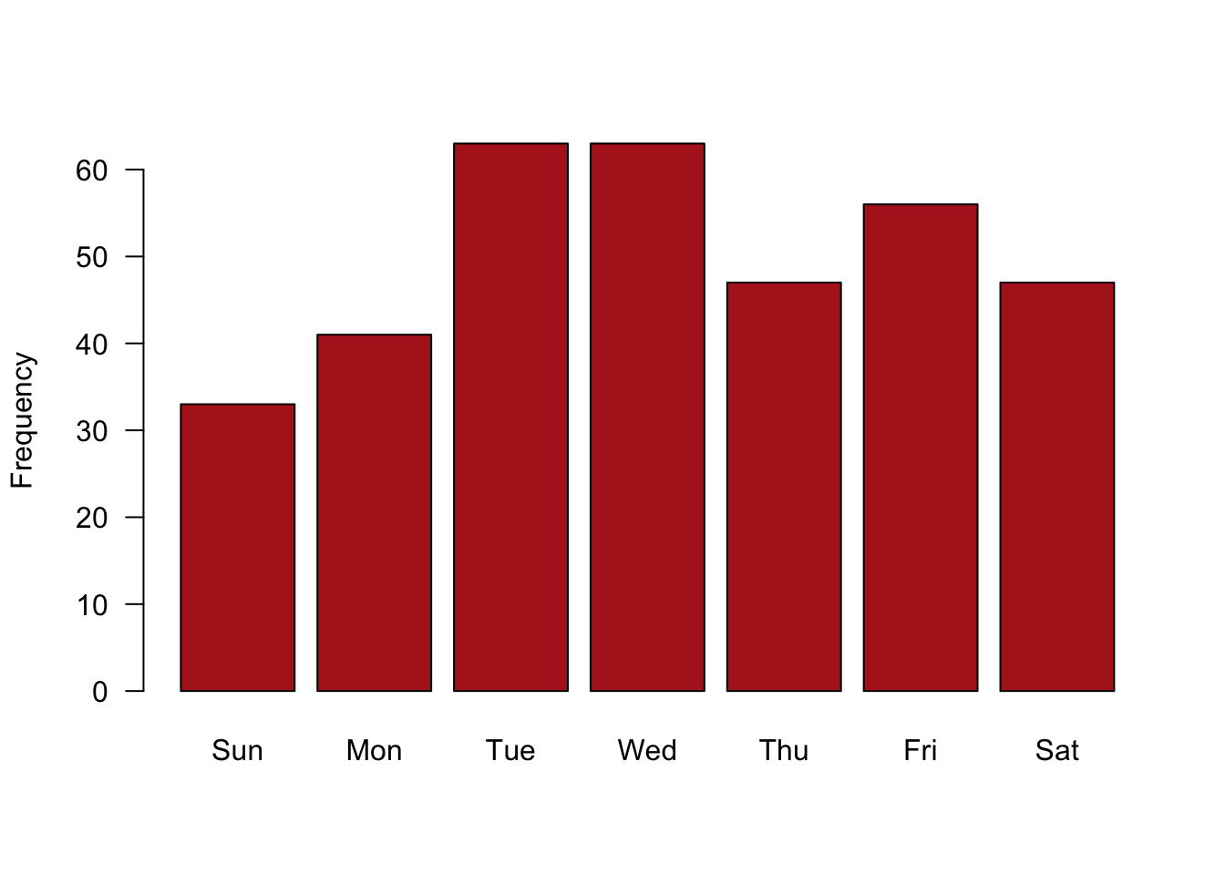
χ2 goodness-of-fit test. The vector p is the expected proportions rather than the expected frequencies, and they must sum to 1 (R nevertheless uses the expected frequencies when calculating the χ statistic). The χ2 value you get here is slightly more accurate than the calculation in the book, which was affected by rounding.
chisq.test(birthDayTable, p = c(52,52,52,52,52,53,52)/365)##
## Chi-squared test for given probabilities
##
## data: birthDayTable
## X-squared = 15.057, df = 6, p-value = 0.01982Example 8.4. Gene content of the human X chromosome
Goodness-of-fit of the proportional model to data with two categories.
Read and inspect the data. Each row is a different gene, with its occurrence on the X chromosome indicated.
geneContent <- read.csv("../Data/chapter08/chap08e4XGeneContent.csv")
head(geneContent)
## chromosome
## 1 X
## 2 X
## 3 X
## 4 X
## 5 X
## 6 XOrder the categories as desired for tables and graphs.
geneContent$chromosome <- factor(geneContent$chromosome, levels = c("X","NotX"))Frequency table showing the number of genes on the X and on other chromosomes.
geneContentTable <- table(geneContent$chromosome)
data.frame(Frequency = addmargins(geneContentTable))
## Frequency.Var1 Frequency.Freq
## 1 X 781
## 2 NotX 19509
## 3 Sum 20290The χ2 goodness-of-fit test to the proportional model.
chisq.test( geneContentTable, p = c(1055, 19235)/20290 )##
## Chi-squared test for given probabilities
##
## data: geneContentTable
## X-squared = 75.065, df = 1, p-value < 2.2e-16The Agresti-Coull 95% confidence interval for the proportion of genes on the X. The command here assumes that you have installed the binom package (see the R pages for Chapter 7).
library(binom)
binom.confint(781, n = 20290, method = "ac")
## method x n mean lower upper
## 1 agresti-coull 781 20290 0.03849187 0.03592951 0.04122894Example 8.5. Designer two-child families?
Goodness-of-fit of the binomial probability model to data on the number of male children in two-child families.
Read and inspect the data. Each row represents a family.
nBoys <- read.csv("../Data/chapter08/chap08e5NumberOfBoys.csv")
head(nBoys)
## numberOfBoys
## 1 0
## 2 0
## 3 0
## 4 0
## 5 0
## 6 0Frequency table of the number of boys in 2-child families.
nBoysTable <- table(nBoys)
data.frame(Frequency = addmargins(nBoysTable))
## Frequency.nBoys Frequency.Freq
## 1 0 530
## 2 1 1332
## 3 2 582
## 4 Sum 2444Estimate the proportion of boys p. Calculate as the mean number of boys in families divided by family size (2).
pHat <- mean(nBoys$numberOfBoys)/2Calculate proportion of families in each category expected under the binomial distribution.
expectedPropFams <- dbinom(0:2, size = 2, prob = pHat)
data.frame(nBoys = c(0,1,2), Proportion = expectedPropFams)
## nBoys Proportion
## 1 0 0.2394749
## 2 1 0.4997737
## 3 2 0.2607515Show the expected number of families in each category under the null hypothesis of a binomial distribution.
data.frame(nBoys = c(0,1,2), Families = expectedPropFams * 2444)## nBoys Families
## 1 0 585.2766
## 2 1 1221.4468
## 3 2 637.2766χ2 goodness-of-fit test. R doesn’t know that you’ve estimated the proportion of boys, the proportion is not specified by the null hypothesis, so it won’t use the correct degrees of freedom. Ignore the P-value that results. Instead, we need to take the χ2 value calculated by chisq.test and recalculate P using the correct degrees of freedom.
saveChiTest <- chisq.test(nBoysTable, p = expectedPropFams)
saveChiTest
##
## Chi-squared test for given probabilities
##
## data: nBoysTable
## X-squared = 20.021, df = 2, p-value = 4.492e-05# Wrong degrees of freedom, wrong P-value! Here's how to make things right:
pValue <- 1 - pchisq(saveChiTest$statistic, df = 1)
pValue## X-squared
## 7.657994e-06Example 8.6. Mass extinctions
Goodness-of-fit of the Poisson probability model to frequency data on number of marine invertebrate extinctions per time block in the fossil record.
Read and inspect the data. Each row is a time block, with the observed number of extinctions listed.
extinctData <- read.csv("../Data/chapter08/chap08e6MassExtinctions.csv")
head(extinctData)
## numberOfExtinctions
## 1 1
## 2 1
## 3 1
## 4 1
## 5 1
## 6 1Generate the frequency table for the number of time blocks in each number-of-extinctions category. Notice that a simple table does what’s needed, but some extinction categories are not represented (e.g., 0, 12 and 13 extinctions).
extinctTable <- table(extinctData$numberOfExtinctions)
data.frame(Frequency = addmargins(extinctTable))
## Frequency.Var1 Frequency.Freq
## 1 1 13
## 2 2 15
## 3 3 16
## 4 4 7
## 5 5 10
## 6 6 4
## 7 7 2
## 8 8 1
## 9 9 2
## 10 10 1
## 11 11 1
## 12 14 1
## 13 16 2
## 14 20 1
## 15 Sum 76To remedy the problem of missing categories, save the original variable as a factor that has all counts between 0 and 20 as levels (note that 20 is not the maximum possible number of extinctions, but it is a convenient cutoff for this table).
extinctData$nExtinctFactor <- factor(extinctData$numberOfExtinctions, levels = c(0:20))
extinctTable2 <- table(extinctData$nExtinctFactor)
data.frame(Frequency = addmargins(extinctTable2))
## Frequency.Var1 Frequency.Freq
## 1 0 0
## 2 1 13
## 3 2 15
## 4 3 16
## 5 4 7
## 6 5 10
## 7 6 4
## 8 7 2
## 9 8 1
## 10 9 2
## 11 10 1
## 12 11 1
## 13 12 0
## 14 13 0
## 15 14 1
## 16 15 0
## 17 16 2
## 18 17 0
## 19 18 0
## 20 19 0
## 21 20 1
## 22 Sum 76Estimate the mean number of extinctions per time block from the data. The estimate is needed for the goodness-of-fit test.
meanExtinctions <- mean(extinctData$numberOfExtinctions)
meanExtinctions
## [1] 4.210526Calculate expected frequencies under the Poisson distribution using the estimated mean. (For now, continue to use 20 extinctions as the cutoff, but don’t forget that the Poisson distribution includes the number-of-extinctions categories 21, 22, 23, and so on.)
expectedProportion <- dpois(0:20, lambda = meanExtinctions)
expectedFrequency <- expectedProportion * 76
Show the frequency distribution in a histogram.
hist(extinctData$numberOfExtinctions, right = FALSE, breaks = seq(0, 21, 1),
    xlab = "Number of extinctions")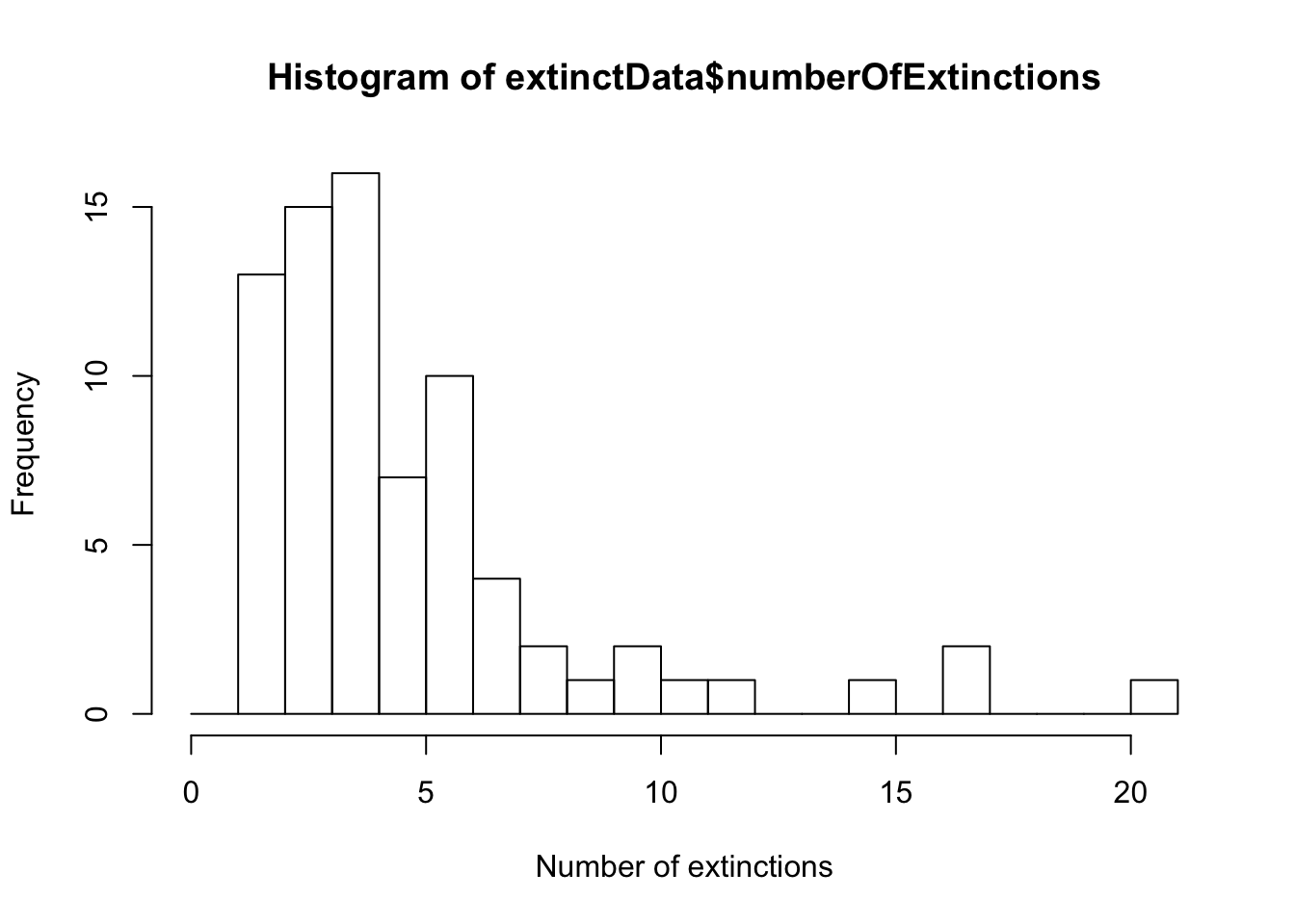
Commands for a fancier histogram, with the expected frequencies overlaid (Figure 8.6-2), are shown here.
# The tricky part is to have the curve overlay the midpoints
#   of the bars, not bar edges, for optimal visual comparison
hist(extinctData$numberOfExtinctions, right = FALSE, breaks = seq(0, 21, 1),
    las = 1, col = "firebrick", xaxt = "n", main = "",
    xlab = "Number of extinctions")
axis(1, at = seq(0.5, 20.5, 1), labels = seq(0,20,1))
lines(expectedFrequency ~ c(0:20 + 0.5), lwd = 2) 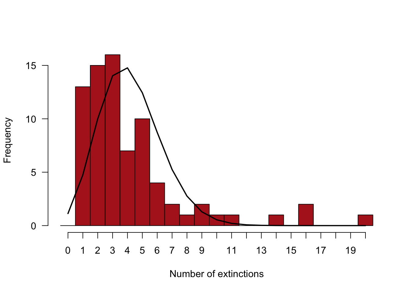
Make a table of observed and expected frequencies, saving as a data frame.
extinctFreq <- data.frame(nExtinct = 0:20, obsFreq = as.vector(extinctTable2),
    expFreq = expectedFrequency)
extinctFreq
## nExtinct obsFreq expFreq
## 1 0 0 1.127730e+00
## 2 1 13 4.748338e+00
## 3 2 15 9.996501e+00
## 4 3 16 1.403018e+01
## 5 4 7 1.476861e+01
## 6 5 10 1.243672e+01
## 7 6 4 8.727524e+00
## 8 7 2 5.249639e+00
## 9 8 1 2.762968e+00
## 10 9 2 1.292616e+00
## 11 10 1 5.442596e-01
## 12 11 1 2.083290e-01
## 13 12 0 7.309790e-02
## 14 13 0 2.367543e-02
## 15 14 1 7.120431e-03
## 16 15 0 1.998718e-03
## 17 16 2 5.259783e-04
## 18 17 0 1.302733e-04
## 19 18 0 3.047328e-05
## 20 19 0 6.753081e-06
## 21 20 1 1.421701e-06The low expected frequencies will violate the assumptions of the χ2 test, so we will need to group categories. Create a new variable that groups the extinctions into fewer categories.
extinctFreq$groups <- cut(extinctFreq$nExtinct,
    breaks = c(0, 2:8, 21), right = FALSE,
    labels = c("0 or 1","2","3","4","5","6","7","8 or more"))
extinctFreq
## nExtinct obsFreq expFreq groups
## 1 0 0 1.127730e+00 0 or 1
## 2 1 13 4.748338e+00 0 or 1
## 3 2 15 9.996501e+00 2
## 4 3 16 1.403018e+01 3
## 5 4 7 1.476861e+01 4
## 6 5 10 1.243672e+01 5
## 7 6 4 8.727524e+00 6
## 8 7 2 5.249639e+00 7
## 9 8 1 2.762968e+00 8 or more
## 10 9 2 1.292616e+00 8 or more
## 11 10 1 5.442596e-01 8 or more
## 12 11 1 2.083290e-01 8 or more
## 13 12 0 7.309790e-02 8 or more
## 14 13 0 2.367543e-02 8 or more
## 15 14 1 7.120431e-03 8 or more
## 16 15 0 1.998718e-03 8 or more
## 17 16 2 5.259783e-04 8 or more
## 18 17 0 1.302733e-04 8 or more
## 19 18 0 3.047328e-05 8 or more
## 20 19 0 6.753081e-06 8 or more
## 21 20 1 1.421701e-06 8 or moreThen sum up the observed and expected frequencies within the new categories.
obsFreqGroup <- tapply(extinctFreq$obsFreq, extinctFreq$groups, sum)
expFreqGroup <- tapply(extinctFreq$expFreq, extinctFreq$groups, sum)
data.frame(obs = obsFreqGroup, exp = expFreqGroup)
## obs exp
## 0 or 1 13 5.876068
## 2 15 9.996501
## 3 16 14.030177
## 4 7 14.768608
## 5 10 12.436722
## 6 4 8.727524
## 7 2 5.249639
## 8 or more 9 4.914760The expected frequency for the last category, “8 or more”, doesn’t yet include the expected frequencies for the categories 21, 22, 23, and so on. However, the expected frequencies must sum to 76. In the following, we recalculate the expected frequency for the last group, expFreqGroup[length(expFreqGroup)], as 76 minus the sum of the expected frequencies for all the other groups.
expFreqGroup[length(expFreqGroup)] = 76 - sum(expFreqGroup[1:(length(expFreqGroup)-1)])
data.frame(obs = obsFreqGroup, exp = expFreqGroup)
## obs exp
## 0 or 1 13 5.876068
## 2 15 9.996501
## 3 16 14.030177
## 4 7 14.768608
## 5 10 12.436722
## 6 4 8.727524
## 7 2 5.249639
## 8 or more 9 4.914761Finally, we are ready to carry out the χ2 goodness-of-fit test. R gives us a warning here because one of the expected frequencies is less than 5. However, we have been careful to meet the assumptions of the χ2 test, so let’s persevere. Once again, R doesn’t know that we’ve estimated a parameter from the data (the mean), so it won’t use the correct degrees of freedom when calculating the P-value. As before, we need to grab the χ2 value calculated by chisq.test and recalculate P using the correct degrees of freedom. Since the number of categories is now 8, the correct degrees of freedom is 8 - 1 - 1 = 6.
saveChiTest <- chisq.test(obsFreqGroup, p = expFreqGroup/76)## Warning in chisq.test(obsFreqGroup, p = expFreqGroup/76): Chi-squared
## approximation may be incorrectsaveChiTest # Wrong degrees of freedom, so wrong P-value!##
## Chi-squared test for given probabilities
##
## data: obsFreqGroup
## X-squared = 23.95, df = 7, p-value = 0.001163pValue <- 1 - pchisq(saveChiTest$statistic, df = 6)
unname(pValue) # correct P-value!## [1] 0.0005334919